Units of Analysis
Intro to Social Science Research
Units of Analysis
Operationalization also depends on our unit of analysis, or the level of social life about which we want to generalize. There are many different such units:
- Individuals
- Groups (families, classes, gangs, …)
- Localities (cities, counties, countries, …)
- Organizations, industries, political units, social artifacts, etc.
For example, consider the concept “poverty.” From Carr et al.:
Counting up the number of economic stressors that a person has faced in the past year (for example, trouble paying bills, getting behind on rent) would be appropriate for categorizing individual people but not neighborhoods. Neighborhood poverty is generally assessed through summary factors that can be more directly and comparably measured across large numbers of people, such as average income. One can try to identify the unit of analysis in a study by asking whether the researchers are trying to compare people to each other or neighborhoods to each other.
Aggregation and Disaggregation
It is possible to operationalize variables at larger units of analysis using variables at smaller units of analysis via a process called aggregation.
Aggregation - “Roll up” a variable measured on a fine-grained unit of analysis (e.g., individuals) into a variable on a coarser-grained unit of analysis (e.g., groups).
- Income of many individuals in geographic regions → average income by region
- Usually done through counting or averaging.
From Carr et al.:
A discussion of historical change in the onset of puberty in the United States occurs at a national level of analysis. Yet, researchers measure that national level by getting data on puberty from individuals and then calculating an average across the group. A country’s average age of puberty is a national-level concept, and its measurement is based on the aggregation of individual-level data.
We will soon see that it can often be challenging to move in the other direction with disaggregation:
Disaggregation: “Drill down” a variable measured on a coarser-grained unit of analysis (e.g., region) into a variable on a coarser-grained unit of analysis (e.g., groups within that region)
- Generally performed to identify confounding (or mediating) variables to disentangle the impact of certain variables (more later)
- Average income by geographic region → average income by race/ethnicity by region
Example Dataset: American Community Survey
Let’s return to our American Community Survey (ACS) 2020 data. It shows education levels of adults 25 years or higher by state.
| State | Estimated total state population | Estimated high school graduate or higher (%) | Estimated bachelor’s degree or higher (%) |
|---|---|---|---|
| Alabama | 3,344,006 | 86.9 | 26.2 |
| California | 26,665,143 | 83.9 | 34.7 |
| Florida | 15,255,326 | 88.5 | 30.5 |
| New York | 13,649,157 | 87.2 | 37.5 |
| Texas | 18,449,851 | 84.4 | 30.7 |
From the ACS webpage, the American Community Survey (ACS) is an ongoing monthly survey that collects detailed housing and socioeconomic data.
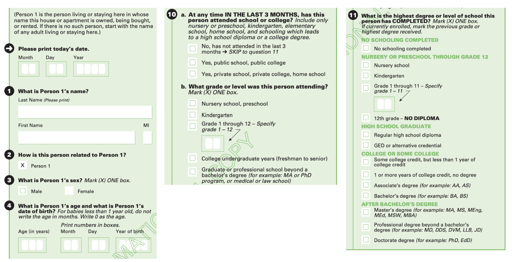
There are (at least) two datasets collected by the ACS: A private dataset of survey responses by household (Figure 1), and a public-facing dataset of responses by geographic region. The variables for the geographic region, a larger unit of analysis, are constructed via aggregation and estimation (Figure 2):
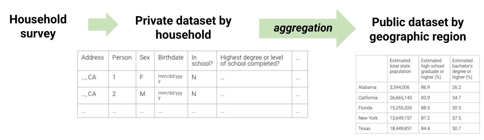
Simple forms of aggregation are straightforward and involve counting and averaging—methods that are very possible using our limited Data Science toolkit thus far. However, disaggregation cannot be done without individual datapoints! There are various methods of estimating individuals from averages using statistics and distributions; we discuss this briefly in a few weeks, but you can take a statistics course for more information.
Privacy and PUMS
Why would the ACS choose to release aggregate data publicly, but keep individual data private? Releasing “fine-grained” data about individuals is a privacy issue. It puts individuals in that dataset at risk of being identified beyond the research. In particular, small, already vulnerable populations are often more easily identified.
Nevertheless, the researchers at ACS understand the value of their government-collected dataset for supporting social science researchers in answering questions about large units of analysis. ACS therefore provides aggregated views of data by region and specific disaggregations by certain demographic factors, such as income and sex.
Researchers who may be studying questions that try to disentangle the impact of demographic factors that ACS disaggregated data does not support (e.g., race/ethnicity) may choose to connect the ACS dataset with a second dataset that has finer-grained data on an individual level, then build up aggregate measures based on differently defined units of analysis.
The ACS Public Use Microdata Sample (PUMS) is one such source. PUMS is a smaller sample of records from individual people and/or housing units that uses a combination of techniques (including differential privacy and synthetic data) to preserve individual privacy (source1, source2). We hope that later in this class we can discuss this privacy protection process.
External Reading
“Chapter 4: From Concepts to Models.” Elizabeth Heger Boyle, Deborah Carr, Benjamin Cornwell, Shelley Correll, Robert Crosnoe, Jeremy Freese, and Waters, Mary C. 2017. The Art and Science of Social Research. New York: W. W. Norton & Company.
References
U.S. Census Bureau, “EDUCATIONAL ATTAINMENT,” American Community Survey 5-Year Estimates Subject Tables, Table S1501, 2020, https://data.census.gov/table/ACSST5Y2020.S1501?q=2020+education&t=Age+and+Sex:Educational+Attainment&g=010XX00US$0400000, accessed on August 24, 2025.
U.S. Census Bureau, “Design and Methodology Report.” https://www.census.gov/programs-surveys/acs/methodology/design-and-methodology.html, accessed on September 2, 2025.
U.S. Census Bureau, “Public Use Microdata Sample (PUMS).” https://www.census.gov/programs-surveys/acs/microdata.html, accessed on September 2, 2025.