Jupyter Notebooks

An introduction to programming

This course uses the Python 3 programming language in the Jupyter Notebook environment. By the end of this note, you’ll understand what that means.

Python 3

From Wikipedia:

A computer program is a [set or sequence] of instructions in a programming language.

Code refers to a computer program written in a particular programming language. In this class, we use the Python 3 programming language. It is powerful and widely used in many computing applications, from web development, scripting, and scientific computing to data science and machine learning. It’s also extremely popular worldwide (Statista, 2025).

Computer programs are nothing more than recipes: we write programs that tell the computer exactly what to do, and it does exactly that—nothing more, and nothing less.

You may be wondering—how can computers be simultaneously so powerful and so primitive? Why does everything in today’s age involve computers or computational technology? In part, this “age of computing” can considered as a complex system of advanced programs run on powerful computing machines to transform complex data. All three of these components involve human scientists and engineers: to write and design the programs, to collect and structure the data, and to design and build the computing machines.

Jupyter Notebooks

In order to run computer programs, we need a way to execute code written in a programming language on a computer. Development, also known as process of designing, iterating, and testing computer programs, often takes place in an environment which can support all of these tasks.

The environment we will use is Jupyter Notebook, which allows us to write and run code within a single .ipynb document (i.e., notebook). They also allow us to embedded text and code.

Figure 1: An example of a Jupyter Notebook.

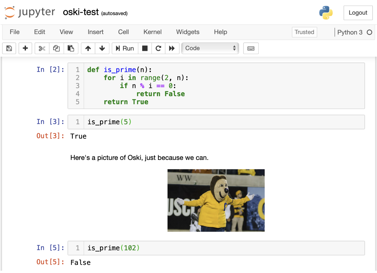
There’s a lot going on in the above Jupyter Notebook screenshot: there is code, there is output from running code, there are pictures, and there is (non-code) text. We’ll get to understanding all of these components in due time.

But this screenshot also elucidates why a tool like Jupyter Notebook is so important to doing data science work. Data Science often requires the use of computation and visualizations and the production of written reports. Notebooks support all three of these, in the same document.

Aside

The Project Jupyter community actually started at UC Berkeley. Professor Fernando Perez of Statistics created an interactive Python environment as part of his graduate studies in Physics, and the rest is history.

Aside 2

Aside 2: Jupyter can run things other than Python—in fact, Jupyter’s namesake is the three core languages it supports: Julia, Python, and R.

If you take more Computer Science and Data Science classes, you will learn about more tools for programming and statistics. In this class we will focus on using Jupyter Notebooks to develop Python code.

DataHub

DataHub is the web-based environment we will use in this course for developing and running Jupyter Notebooks. Some features:

• DataHub is a Berkeley-hosted server that runs Jupyter notebooks.
• All students have their own DataHub “container”; think of this as your own virtual computer.
• This is where you will work on all assignments.
• You will not need to install anything locally (meaning that you could theoretically do all assignments for this class on your phone, but we recommend giving your fingers and your eyes a break). All you need is a web browser.
• Course staff can access everything in your DataHub to help debug your code.

Access DataHub

In this class, there are two common ways to develop Jupyter Notebooks:

1. Go to http://datahub.berkeley.edu. Make a new notebook, or open an existing one.
2. From our course website, often by clicking on code links or assignment links. These will often create a copy of a notebook skeleton, which you can then run or edit.

Generally, we will not be creating notebooks from scratch. Instead, the course staff have helped write scaffolding code and instructions for activities that are designed to help you understand the fundamentals.

Jupyter Notebook Internals

Caution

If you have not yet tried interacting with your first Jupyter Notebook yet, this section will not make much sense. We recommend skipping ahead to the next set of notes, then coming back and referring to this as you build more notebooks.

Jupyter Notebooks are made up of cells. There are two main types of cells:

Code cells. This is where you write and execute code. When run, Python code cells are evaluated as a Python code snippet, one line at a time. The cell output displayed is the value of the last evaluated expression:

Figure 2: Both expressions are evaluated, but the result of the last expression’s evaluation is considered the output of the code cell.

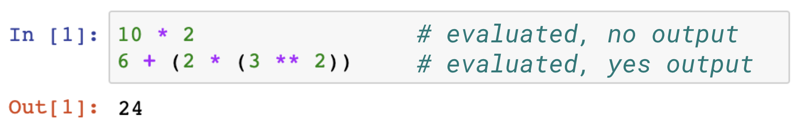
We will discuss this output/display phenomenon more in future notes.

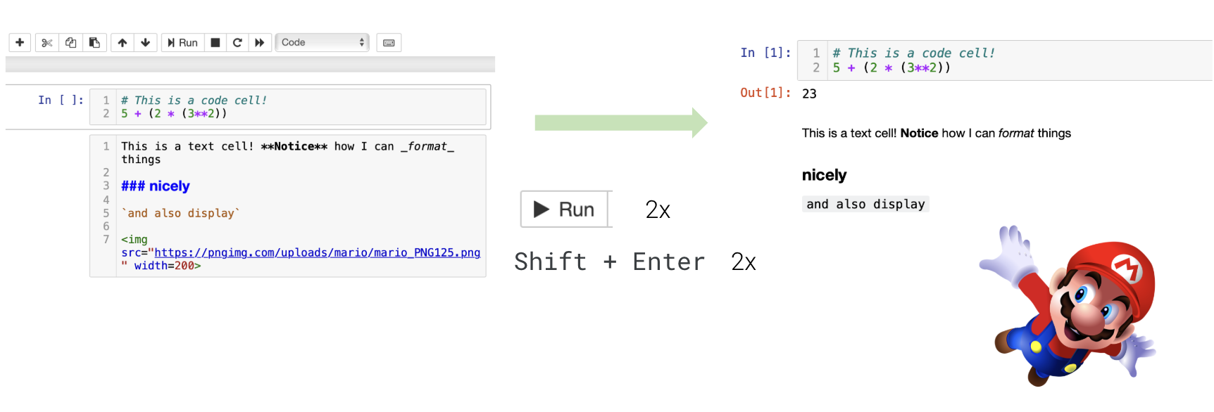
To run a code cell, you can either hit the “Run” button in the Toolbar, or you can use a keyboard shortcut: <SHIFT>+<ENTER>, which runs the cell and advances to the next cell. We recommend keyboard shortcuts; see below.

Markdown cells. This is where you write text and images that aren’t Python code. Markdown is a language used for formatting text. A Markdown cell will always display its formatting when it is not in edit mode.

Figure 3: Left screenshot shows un-evaluated code cell and raw Markdown cell; right screenshot shows evaluated code cell and formatted text. To render formatted text for a selected markdown cell, exit editing mode for that cell. This screenshot starts with the code cell selected, then runs both that code cell and “runs” the markdown cell below.

Here is a guide to Markdown formatting. You’ll explore Markdown more in lab.

Keyboard Shortcuts

While you can manage most of your notebook development by leveraging the Toolbar, many programmers (including me!) prefer using keyboard shortcuts. This minimizes use of the mouse/trackpad and keeps the hands on the keyboard. Together with stretching and taking breaks, keyboard shortcuts will reduce wrist cramps and improve your programming concentration.

Edit mode vs. command mode: Hit the <ESCAPE> key on your keyboard to switch from edit mode to command mode. Keyboard shortcuts are specific to the mode you’re using:

• Edit mode: when you’re actively typing in the cell. Undo is <CTRL/CMD> + Z.
• Command mode: when you’re not actively typing in the cell. Undo is z.

Action	Mode	Keyboard shortcut
Run cell + jump to next cell*	Either (puts you in edit mode)	<SHIFT> + <ENTER>
Run cell + stay on this cell	Either (puts you in edit mode)	<CTRL/CMD> + <ENTER>
Save notebook	Either	<CTRL/CMD> + <S>
Switch to command mode*	Either (puts you in command mode)	<ESCAPE>
Switch to edit mode*	Command	<ENTER>
Comment out the current line	Edit	<CTRL/CMD> + /
Create new cell above/below	Command	A/B
Delete cell	Command	DD
Convert cell to Markdown	Command	M
Convert cell to code	Command	Y
Show all shortcuts	Command	H

The above table should be used as a reference throughout the semester; don’t try to memorize these right now. And remember, you don’t have to use these shortcuts; you can always use the toolbar. Regardless, we’ve annotated the most useful keyboard shortcuts with an asterisk (*).

There are plenty more keyboard shortcuts available. Let us know if you find a good guide.